Using quantized data types

High-resolution simulations can deliver great visual quality, but they are often limited by available memory, especially on GPUs. For the sake of saving memory, Taichi provides low-precision ("quantized") data types. You can define your own integers, fixed-point numbers or floating-point numbers with non-standard number of bits so that you can choose a proper setting with minimum memory for your applications. Taichi provides a suite of tailored domain-specific optimizations to ensure the runtime performance with quantized data types close to that with full-precision data types.

note

Quantized data types are only supported on CPU and CUDA backends for now.

Quantized data types

Quantized integers

Modern computers represent integers using the two's complement format. Quantized integers in Taichi adopt the same format, and can contain non-standard number of bits:

i10 = ti.types.quant.int(bits=10)  # 10-bit signed (default) integer type
u5 = ti.types.quant.int(bits=5, signed=False)  # 5-bit unsigned integer type

Quantized fixed-point numbers

Fixed-point numbers are an old way to represent real numbers. The internal representation of a fixed-point number is simply an integer, and its actual value equals to the integer multiplied by a predefined scaling factor. Based on the support for quantized integers, Taichi provides quantized fixed-point numbers as follows:

fixed_type_a = ti.types.quant.fixed(bits=10, max_value=20.0)  # 10-bit signed (default) fixed-point type within [-20.0, 20.0]
fixed_type_b = ti.types.quant.fixed(bits=5, signed=False, max_value=100.0)  # 5-bit unsigned fixed-point type within [0.0, 100.0]
fixed_type_c = ti.types.quant.fixed(bits=6, signed=False, scale=1.0)  # 6-bit unsigned fixed-point type within [0, 64.0]

scale is the scaling factor mentioned above. Because fixed-point numbers are especially useful when you know the actual value is guaranteed to be within a range, Taichi allows you to simply set max_value and will calculate the scaling factor accordingly.

Quantized floating-point numbers

Floating-point numbers are the standard way to represent real numbers on modern computers. A floating-point number is composed of exponent bits, fraction bits, and a sign bit. There are various floating-point formats:

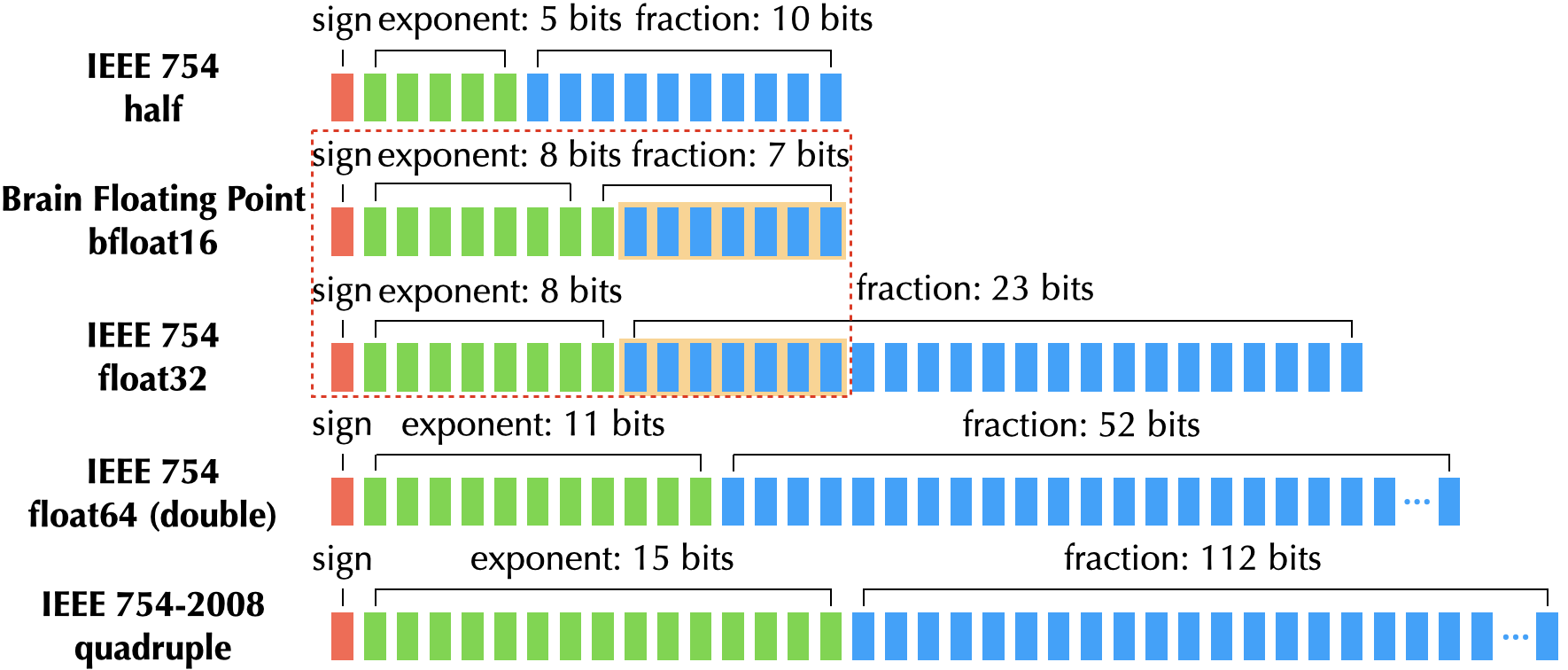
In Taichi, you can define a quantized floating-point number with arbitrary combination of exponent bits and fraction bits (the sign bit is made part of fraction bits):

float_type_a = ti.types.quant.float(exp=5, frac=10)  # 15-bit signed (default) floating-point type with 5 exponent bits
float_type_b = ti.types.quant.float(exp=6, frac=9, signed=False)  # 15-bit unsigned floating-point type with 6 exponent bits

Compute types

All the parameters you've seen above are specifying the storage type of a quantized data type. However, most quantized data types have no native support on hardware, so an actual value of that quantized data type needs to convert to a primitive type ("compute type") when it is involved in computation.

The default compute type for quantized integers is ti.i32, while the default compute type for quantized fixed-point/floating-point numbers is ti.f32. You can change the compute type by specifying the compute parameter:

i21 = ti.types.quant.int(bits=21, compute=ti.i64)
bfloat16 = ti.types.quant.float(exp=8, frac=8, compute=ti.f32)

Data containers for quantized data types

Because the storage types are not primitive types, you may now wonder how quantized data types can work together with data containers that Taichi provides. In fact, some special constructs are introduced to eliminate the gap.

Bitpacked fields

ti.BitpackedFields packs a group of fields whose dtypes are quantized data types together so that they are stored with one primitive type. You can then place a ti.BitpackedFields instance under any SNode as if each member field is placed individually.

a = ti.field(float_type_a)  # 15 bits
b = ti.field(fixed_type_b)  # 5 bits
c = ti.field(fixed_type_c)  # 6 bits
d = ti.field(u5)  # 5 bits
bitpack = ti.BitpackedFields(max_num_bits=32)
bitpack.place(a, b, c, d)  # 31 out of 32 bits occupied
ti.root.dense(ti.i, 10).place(bitpack)

Shared exponent

When multiple fields with quantized floating-point types are packed together, there is chance that they can share a common exponent. For example, in a 3D velocity vector, if you know the x-component has a much larger absolute value compared to y- and z-components, then you probably do not care about the exact value of the y- and z-components. In this case, using a shared exponent can leave more bits for components with larger absolute values. You can use place(x, y, z, shared_exponent=True) to make fields x, y, z share a common exponent.

Your first program

You probably cannot wait to write your first Taichi program with quantized data types. The easiest way is to modify the data definitions of an existing example. Assume you want to save memory for examples/simulation/euler.py. Because most data definitions in the example are similar, here only field Q is used for illustration:

Q = ti.Vector.field(4, dtype=ti.f32, shape=(N, N))

An element of Q now occupies 4 x 32 = 128 bits. If you can fit it in 64 bits, then the memory usage is halved. A direct and first attempt is to use quantized floating-point numbers with a shared exponent:

float_type_c = ti.types.quant.float(exp=8, frac=14)
Q_old = ti.Vector.field(4, dtype=float_type_c)
bitpack = ti.BitpackedFields(max_num_bits=64)
bitpack.place(Q_old, shared_exponent=True)
ti.root.dense(ti.ij, (N, N)).place(bitpack)

Surprisingly, you find that there is no obvious difference in visual effects after the change, and you now successfully finish a Taichi program with quantized data types! More attempts are left to you.

More complicated quantization schemes

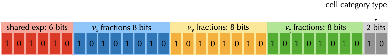
Here comes a more complicated scenario. In a 3D Eulerian fluid simulation, a voxel may need to store a 3D vector for velocity, and an integer value for cell category with three possible values: "source", "Dirichlet boundary", and "Neumann boundar". You can actually store all information with a single 32-bit ti.BitpackedFields:

velocity_component_type = ti.types.quant.float(exp=6, frac=8, compute=ti.f32)
velocity = ti.Vector.field(3, dtype=velocity_component_type)

# Since there are only three cell categories, 2 bits are enough.
cell_category_type = ti.types.quant.int(bits=2, signed=False, compute=ti.i32)
cell_category = ti.field(dtype=cell_category_type)

voxel = ti.BitpackedFields(max_num_bits=32)
# Place three components of velocity into the voxel, and let them share the exponent.
voxel.place(velocity, shared_exponent=True)
# Place the 2-bit cell category.
voxel.place(cell_category)
# Create 512 x 512 x 256 voxels.
ti.root.dense(ti.ijk, (512, 512, 256)).place(voxel)

The compression scheme above allows you to store 13 bytes (4B x 3 + 1B) into just 4 bytes. Note that you can still use velocity and cell_category in the computation code, as if they are ti.f32 and ti.u8.

Quant arrays

Bitpacked fields are actually laid in an array of structure (AOS) order. However, there are also cases where a single quantized type is required to get laid in an array. For example, you may want to store 8 x u4 values in a single u32 type, to represent bin values of a histogram:

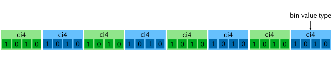
Quant array is exactly what you need. A quant_array is a SNode which can reinterpret a primitive type into an array of a quantized type:

bin_value_type = ti.types.quant.int(bits=4, signed=False)

# The quant array for 512 x 512 bin values
array = ti.root.dense(ti.ij, (512, 64)).quant_array(ti.j, 8, max_num_bits=32)
# Place the unsigned 4-bit bin value into the array
array.place(bin_value_type)

note

1. Only one field can be placed under a quant_array.
2. Only quantized integer types and quantized fixed-point types are supported as the dtype of the field under a quant_array.
3. The size of the dtype of the field times the shape of the quant_array must be less than or equal to the max_num_bits of the quant_array.

Bit vectorization

For quant arrays of 1-bit quantized integer types ("boolean"), Taichi provides an additional optimization - bit vectorization. It aims at vectorizing operations on such quant arrays under struct fors:

u1 = ti.types.quant.int(1, False)
N = 512
M = 32
x = ti.field(dtype=u1)
y = ti.field(dtype=u1)
ti.root.dense(ti.i, N // M).quant_array(ti.i, M, max_num_bits=M).place(x)
ti.root.dense(ti.i, N // M).quant_array(ti.i, M, max_num_bits=M).place(y)

@ti.kernel
def assign_vectorized():
    ti.loop_config(bit_vectorize=True)
    for i, j in x:
        y[i, j] = x[i, j]  # 32 bits are handled at a time

assign_vectorized()

Advanced examples

The following examples are picked from the QuanTaichi paper, so you can dig into details there.

Game of Life

Eulerian Fluid

MLS-MPM